
Sacramento Transit - Part 1 - Exploration
Background
As cities become increasingly concerned about traffic, infrstructure maintainence, and the environment; increased use of public transit could be way to address several of these challenges at once. I've become interested in understanding how cities can address these challenges, and began reading about urban planning a few years ago. Through reading what some long-time urban planners have to say, I'm beginning to see that if increasing public transit can help alleviate traffic, maintenance and environmental issues, increasing ridership is a multi-dimensional challenge in its own right. The way many places are organized, daily and individual car use is practically required due to the way that most activites and ammenities are spread over miles and metro areas and frequently aren't connected by transit networks.
As I've been reading about urban planning, public transportation, and urban informatics in the past few years, these are the sources that I keep coming back to:
- Human Transit (https://humantransit.org/)
- Strong Towns (https://www.strongtowns.org)
- Parking and the City (https://www.shoupdogg.com/)
- Blog of, Geoff Boeing, Professor of Urban Informatics at Northwestern (https://geoffboeing.com/)
To summarize what I've learned from reading these: an effort to increase public transit ridership would have to address many different dimensions of residents' experience as they choose their preferred mode of travel on a regular basis. Some of these are physical characteristics of the public transit network, that also overlap with perceptions of the transit network, and chances are both types will need to be addressed at every step:
- Is public transit nearby?
- Is it safe and easy to get there?
- Does it arrive frequently, or will it be a long wait?
- Does it go where residents need to go?
- Does it get there quickly (compared with other options)?
- Is it cost efficient, and comfortable compared with other options?
- Are residents aware that public transit is a nearby option that frequently goes where they need to go?
Introduction
Using some open data and open-source libraries, we can begin by asking some of the higher level questions around availability.
- For how many people is public transit nearby and easy to get to?
- What are ways that a city can increase the percentage of the population that are in close and easy access to public transit?
In this series of posts I'll be using some publically available data to explore the new transit plans in Sacramento, CA including where current and proposed stops are located, and what the density and zoning of the areas around those stops currently are.
The following blog posts, motivated me to explore some of these questions in Sacramento. In addition, Sacramento has a great open data website, with lots of useful publically available datasets that anyone can use to analyze the transit network.
- https://www.strongtowns.org/journal/2019/1/17/new-planning-paradigm-sacramento
- https://www.strongtowns.org/journal/2018/11/28/a-suburban-model-for-incremental-transit
- https://humantransit.org/2011/04/basics-walking-distance-to-transit.html
Methods and Datasets
To explore Sacramento's transit plan, I've obtained several open datasets from their open data portal (http://data.cityofsacramento.org/)
- Current and newly planned transit stops (Shapefile)
- neighborhoods (Shapefile)
- Zoning Areas (Shapefile)
In future exploration, I'll look at the street walking network near the stops as well as estimated number of households near the stops.
First question to explore in Part 1
- What kinds zoning areas are located near current and planned transit stops? ( Focusing on rail )
I'll be doing all of this work using open data, and python's geopandas library, making the maps and the exploratory analysis very reproducable.
I do not have traning as an urban planner, but using the open data that I have access to and some principles from my reading, I'll try to put myself in the mindset of a planner who is interested in increasing the percentage of trips that happen using public transit.
0. Setup for replicating this analysis
First of all, I want to make the maps and exploratory analysis as replicable as possible.
If you want to run through this notebook/analysis yourself, you can, because it uses open data and open source tools. It's especially easy if you have docker https://docs.docker.com/docker-for-mac/. Because that means that you don't have to install python or the specific libraries I'm using in the post, since they will already come packaged in the docker container.
If you have docker installed, you would run one of these sets of commands at the command line to create the environment that you need for running the rest of this notebook:
# Geospaital jupyter notebook.

> cd [location of this notebook]
> docker run -p 8888:8888 -v "$PWD":/home/jovyan/work gboeing/osmnx
# Basic jupyter notebook. You'll still need to install geospatial libraries (geopandas)
> cd [location of this notebook]
> docker run -p 8888:8888 -v "$PWD":/home/jovyan/work jupyter/scipy-notebook#! pip install geopandas # If you need to install geopandas
# Todo: #! pip install contextily # https://github.com/darribas/contextily
import geopandas as gpd
import pandas as pd
import requests
import tempfile

# Show the plots in the notebook
%matplotlib inline

# Don't show warnings from the libraries
import warnings
warnings.filterwarnings('ignore')

# How to format numbers in the tables
pd.options.display.float_format = '{:20,.2f}'.format
1. Find Some Data
Load and explore a few datasets that may be relevant from the Sacramento open data portal. (http://data.cityofsacramento.org/)
- Current and newly planned transit stops (Shapefile)
- Sacramento neighborhoods (Shapefile)
- Zoning Areas (Shapefile), which describe what kinds of buildings and uses are allowed in different parts of the city.
def shp_api_loader(url):
    response = requests.get(url)

    with tempfile.NamedTemporaryFile() as f:
        f.write(response.content)
        return gpd.read_file(f.name)
Neighborhoods
#Read Neighborhoods Shapes
url = 'https://opendata.arcgis.com/datasets/49f20f1612ae4f0a9292eb65f8bd4013_0.geojson'
nb = shp_api_loader(url)
nb.plot()

Zoning Areas
url = 'https://opendata.arcgis.com/datasets/13a456d86b0d47459a61e2dacfc8f609_0.geojson'
zone = shp_api_loader(url)
print(zone.head(2))
Top zones by area
zone_sizes = zone.groupby('ZONE')['Shape__Area'].agg({'area': 'sum','count': len})
zone_sizes.sort_values('area', ascending = False).head(10)
top_5_zones_by_area = zone_sizes.sort_values('area', ascending = False).head(5).index.tolist()
base = nb.to_crs(epsg =26946).plot( figsize = (10,10),
                                    color = 'lightgrey', alpha = 0.5, edgecolor = 'black')

zone[zone.ZONE.isin(top_5_zones_by_area)].to_crs(epsg =26946).plot(
    column='ZONE', legend = True, cmap = 'viridis',
    ax = base)

_ = base.axis('off')

_ = base.set_title("Top 5 zoning types, by area")

Transit Stops ( Bus and Rail )
Observations
- The bus stops dataset doesn't appear to show what line it's on. Bus lines data would be required to figure out where the buses at each stop can take you.
# Bus Stops ( Sacramento regional area )
url = 'https://opendata.arcgis.com/datasets/de9ea608eefb4214ae5f4897181a3d03_0.geojson'
bus_stops = shp_api_loader(url)

print(bus_stops.head(2))
bus_stops.plot()

# SRT Light Rail rail stops
url = 'https://opendata.arcgis.com/datasets/247bcd4bd2504967a13271ed0f749fe4_0.geojson'
rail_stops =shp_api_loader(url)

print(rail_stops.head(2))
rail_stops.plot()

# future light rail
# https://hub.arcgis.com/datasets/8d8896143666437daa78e47aa05e7ee2_0
url = 'https://opendata.arcgis.com/datasets/8d8896143666437daa78e47aa05e7ee2_0.geojson'
rail_stops_f =shp_api_loader(url)

#print(rail_stops_f.head(2))
rail_stops_f.plot()
rail_stops_f['future'] = 'planned'

rail_stops['future'] = 'current'
all_rail = gpd.GeoDataFrame(pd.concat([rail_stops, rail_stops_f]))
all_rail.crs = rail_stops.crs
all_rail.plot(column = 'future', legend = True)

2. Explore where transit, neighborhoods, and zoning types overlap
Data Processing Steps:
- https://epsg.io/26946 : 800 Meters in a half mile
- Subset the transit stops to the 'Sacramento Neighborhoods' shapes.
- Find areas within a 0.25 mi and 0.5 miles buffer of a transit stop ( This is the area that the book, Human Transit would say is within a reasonable walking distance for frequent use )
Key Observations:
- A very high proportion of the city's area is within a 0.5 mile of a bus stop, however, according to Human Transit, a sufficient network and frequency is also necessary for access to bus stops to be efficient for residents' primary transportation needs. Since I don't currently have data that can be used to determine where the bus stops go, and how frequently they arrive I'll be focusing on rail for now.
base = nb.to_crs(epsg =26946).plot( figsize = (10,6),
                                    color = 'lightgrey', alpha = 0.5, edgecolor = 'black')
gpd.sjoin(all_rail, nb[['geometry']], how = 'inner').to_crs(epsg =26946).plot(
                ax = base,
                column = 'future',
                markersize = 10,
                legend = True,
                cmap = 'viridis'
               )

_ = base.axis('off')

_ = base.set_title("Transit stop locations (Current and Planned)")

base = nb.to_crs(epsg =26946).plot(figsize=(10,10), color = 'lightgrey', alpha = 0.5, edgecolor = 'black')

gpd.sjoin(all_rail[all_rail.future =='current'], nb[['geometry']], how = 'inner').to_crs(epsg =26946).geometry.buffer(800).plot(
                ax = base,
                color = 'orange',
                alpha = 0.7
               )
gpd.sjoin(all_rail[all_rail.future =='current'], nb[['geometry']], how = 'inner').to_crs(epsg =26946).geometry.buffer(400).plot(
                ax = base,
                color = 'red',
                alpha = 0.7
               )
_ = base.axis('off')

_ = base.set_title("Current area within 0.5 or 0.25 miles of a transit stop")

base = nb.to_crs(epsg =26946).plot(figsize=(10,10),
                                   color = 'lightgrey', alpha = 0.5, edgecolor = 'grey')

gpd.sjoin(all_rail, nb[['geometry']], how = 'inner').to_crs(epsg =26946).geometry.buffer(800).plot(
                ax = base,
                color = 'orange',
                alpha = 0.7
               )
gpd.sjoin(all_rail, nb[['geometry']], how = 'inner').to_crs(epsg =26946).geometry.buffer(400).plot(
                ax = base,
                color = 'red',
                alpha = 0.7
               )
_ = base.axis('off')

_ = base.set_title("Current and Planned area within 0.5 or 0.25 miles of a transit stop")

Bus Stops
Key Observations
- Lots of the city is within walking distance of an existing bus stop.
- Without further information about where the bus stops go, and how they connect to other transit and areas of town, it's hard to know if the bus routes go where people need them to, frequently.
base = nb.to_crs(epsg =26946).plot(figsize=(10,10),
                                   color = 'lightgrey',
                                   alpha = 0.5,
                                   edgecolor = 'grey')

gpd.sjoin(bus_stops, nb[['geometry']], how = 'inner').to_crs(epsg =26946).geometry.buffer(800).plot(
                ax = base,
                color = 'orange',
                alpha = 0.7
               )
gpd.sjoin(bus_stops, nb[['geometry']], how = 'inner').to_crs(epsg =26946).geometry.buffer(400).plot(
                ax = base,
                color = 'red',
                alpha = 0.7
               )
_ = base.axis('off')

_ = base.set_title("Current area within 0.5 miles of a bus stop")

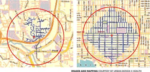
What if we assume a walkable grid
To fit closer with how people are going to experience the city, it's better to assume a 'Grid' configuration for the walking blocks https://humantransit.org/2011/04/basics-walking-distance-to-transit.html , and use a square rather than a circle to estimate the area that's within 0.25 to 0.5 miles walk-ing distance.
This is still an optimistic view of how far people can walk, since street layouts that are not grids are common in many cities, and are often less efficient for walking.
Creating a function for creating a 'square' inscribed within the desired radius
import math

def inscribe_square(points,
                    buffer_circle = 400, # https://epsg.io/26946 :  800 Meters is approx a half mile
                    orientation_radians = (1/4), # pi/4 is 90 degree rotation
                    show=False # If show = True, make a plot, if false, just return the polygons
                   ):

    # pythagorean theorem
    square_len = ((buffer_circle**2)/2)**0.5
    if show:
        print("inscribed square leg width approx: {0}, for buffer radius: {1}".format(square_len, buffer_circle))

    inner_circle = points.buffer(square_len)
    outer_circle = points.buffer(buffer_circle)
    inscribed_square = inner_circle.envelope.rotate(
                            angle = math.pi*orientation_radians, use_radians=True)

    if show:
        base = outer_circle.plot(color = 'purple')
        inscribed_square.plot(ax = base, color = 'grey')
        inner_circle.plot(ax = base, color = 'blue')

    return inscribed_square


inscribe_square(
    gpd.sjoin(all_rail[all_rail.future =='current'], nb[['geometry']], how = 'inner'
             ).to_crs(epsg =26946
                 ).geometry[2:10],
    show=True
)

base = nb.to_crs(epsg =26946).plot(figsize=(10,10),
                                   color = 'lightgrey', alpha = 0.5,
                                   edgecolor = 'grey')

inscribe_square(
            gpd.sjoin(all_rail[all_rail.future =='current'],
                      nb[['geometry']],
                      how = 'inner'
             ).to_crs(epsg =26946
                     ).geometry,
                 buffer_circle = 800
             ).plot(figsize=(10,10), color = 'orange', ax = base)

inscribe_square(
             gpd.sjoin(all_rail[all_rail.future =='current'],
                       nb[['geometry']],
                       how = 'inner'
             ).to_crs(epsg =26946
                     ).geometry,
             buffer_circle = 400).plot(color= 'red', ax = base)


_ = base.axis('off')

_ = base.set_title("Current area within 0.5 miles walking grid of a transit stop")

3. Exploratory Question
A) What types of zoned areas are within walking distance of current and planned transit?
Zoning rules determine what kinds of structures and uses are allowed to be in certain parts of a city.
The top zoning codes by area, when looking at the city's zoning dataset are:
R-1: Standard Single-Family Zone: This is a low density residential zone composed of single-family, detached residences on lots a minimum of fifty-two (52) feet by one hundred (100) feet in size. A duplex or a half-plex is allowed on a corner lot subject to compliance with development standards. Residential neighborhoods are commonly zoned this way.
R-3: Multi-Family Zone: This is a multi-family residential zone intended for more traditional types of apartments.
C-2: General Commercial Zone: This is a general commercial zone which provides for the sale of commodities, or performance of services, including repair facilities, offices, small wholesale stores or distributors, and limited processing and packaging. Good examples are a small neighborhood hardware store or a corner market.
M-2: Heavy Industrial Zone: This zone permits the manufacture or treatment of goods from raw materials.
A: Agricultural Zone: This is an agricultural zone restricting the use of land primarily to agriculture and farming.
Currently, I don't have a complete list of the zoning codes in the dataset, however the webpage linked above gives an idea of what the codes mean, in particular:
- R-1, appears to be some variation of single-family and low-density residential
- R-3, appears to be some variation of traditional multi-family or higher-density residential
base = nb.to_crs(epsg =26946).plot(figsize=(10,10),
                                   color = 'lightgrey', alpha = 0.5,
                                   edgecolor = 'grey')

inscribe_square(
            gpd.sjoin(all_rail[all_rail.future =='current'], nb[['geometry']], how = 'inner'
             ).to_crs(epsg =26946
                     ).geometry,
                 buffer_circle = 800
             ).plot(figsize=(10,10), color = 'orange', ax = base)

inscribe_square(
             gpd.sjoin(all_rail[all_rail.future =='current'], nb[['geometry']], how = 'inner'
             ).to_crs(epsg =26946
                     ).geometry,
             buffer_circle = 400).plot(color= 'red', ax = base)

zone[zone.ZONE.isin(top_5_zones_by_area)].to_crs(epsg =26946).plot(
    column='ZONE', legend = True, cmap = 'viridis',
    alpha = 0.5,
    ax = base)


_ = base.axis('off')

_ = base.set_title("Top 5 zoning types city-wide")

all_rail_in_nb = gpd.sjoin(all_rail, nb[['geometry']], how = 'inner')
all_rail_in_nb['stop_geometry']=all_rail_in_nb.geometry
all_rail_in_nb['inscribed_half_mile_square'] = inscribe_square(
         all_rail_in_nb.to_crs(epsg =26946).geometry,
                 buffer_circle = 800
             )
all_rail_in_nb.geometry = all_rail_in_nb.inscribed_half_mile_square
all_rail_in_nb = all_rail_in_nb[['ACTIVE', 'NAME', 'NODE', 'STOP_NAME','future', 'stop_geometry', 'inscribed_half_mile_square','geometry']]
base = zone.to_crs(epsg =26946).plot()

all_rail_in_nb.head().plot(ax = base, color = 'red')

base = gpd.overlay(all_rail_in_nb.head(),
            zone.to_crs(epsg =26946),
            how='intersection').plot(figsize = (12,12),
                                     column = 'ZONE',
                                     legend = True)

_ = base.axis('off')

_ = base.set_title("Zones that are near transit stops")

zones_near_transit = gpd.overlay(
            all_rail_in_nb,
            zone.to_crs(epsg =26946),
            how='intersection')

base = zones_near_transit.plot(column = 'ZONE')

_ = base.axis('off')

_ = base.set_title("Zones that are near transit stops")

Top five zones by area near transit
# Calculate the area of the zoned shape, after it's been subsetted to the area near transit
zones_near_transit['area_near_transit'] = zones_near_transit.geometry.area
zones_near_transit_counts = zones_near_transit.groupby('ZONE').area_near_transit.agg(
    {'area': 'sum','count': len}
).sort_values('area', ascending = False)

zones_near_transit_counts.head(5)
base = all_rail_in_nb.plot(figsize = (10,10),
                           #column = 'future',
                           color = 'lightgrey',
                           alpha = 0.5)

all_rail_in_nb[all_rail_in_nb.future == 'current'].plot(
                    ax = base,
                    color = 'Grey',
                    alpha = 0.5)

zones_near_transit[zones_near_transit.ZONE.isin(zones_near_transit_counts.head(5).index.tolist())
                  ].plot(ax = base,
                         column = 'ZONE',
                         legend = True,
                         cmap = 'plasma')


_ = base.axis('off')

_ = base.set_title("Top 5 zoning types, within 0.5 miles walking grid of a transit stop")

## Functions

def calculate_top_zones(zones_df, highlight_stops):
    top_zones_near_highlight_stop = zones_df[zones_df.STOP_NAME.isin(highlight_stops)]

    top_zones_near_highlight_stop['zone_area'] = top_zones_near_highlight_stop.geometry.area

    top_zones_near_highlight_stop = top_zones_near_highlight_stop.groupby('ZONE').zone_area.agg(
        {'area': 'sum','count': len}
    ).sort_values('area', ascending = False)

    top_zones_near_highlight_stop['pct_area'] = top_zones_near_highlight_stop.area/top_zones_near_highlight_stop.area.sum()
    return top_zones_near_highlight_stop


def plot_zones_near_highlight(rail_stops,
                              zones_near_stops,
                              highlight_stop, top_n = 5):

    # Grey Background for the area around the stop
    base = rail_stops[rail_stops.STOP_NAME.isin(highlight_stop)].plot(
                           figsize = (10,10),
                           color = 'lightgrey',
                           alpha = 0.5)
    if top_n is None:
        top_n_filter = True
        top_n_label = ''
    else:
        top_zones_near_highlight_stop = calculate_top_zones(zones_near_stops, highlight_stop)
        top_n_filter = (zones_near_transit.ZONE.isin(top_zones_near_highlight_stop.head(top_n).index.tolist()))
        top_n_label = "Top {}".format(top_n)

    # Zones
    zones_near_stops[(zones_near_stops.STOP_NAME.isin(highlight_stop))
                      & top_n_filter
                      ].plot(ax = base,
                             column = 'ZONE',
                             legend = True,
                             cmap = 'plasma')

    # Stop point in Red
    stop_points = gpd.GeoDataFrame({'geometry': rail_stops[rail_stops.STOP_NAME.isin(highlight_stop)].stop_geometry}
                     )
    stop_points.crs = rail_stops.crs
    stop_points.to_crs(epsg =26946).plot(ax = base,
                           color = 'red',
                           markersize = 200
    )

    _ = base.axis('off')

    _ = base.set_title("{topn} Zoning types, within 0.5 miles walking grid of: \n {stops}".format(topn = top_n_label,
                                                                                                  stops = ";".join(highlight_stop)) )

    return base
highlight_stop = all_rail_in_nb.STOP_NAME.head(20).tail(3).tolist()

calculate_top_zones(zones_near_transit, highlight_stop).head()

myplt = plot_zones_near_highlight(all_rail_in_nb,
                                  zones_near_transit,
                                  highlight_stop, top_n = 10)

calculate_top_zones(zones_near_transit,
                    highlight_stop).head(10)

highlight_stop = ['Roseville Road']


myplt = plot_zones_near_highlight(all_rail_in_nb,
                                  zones_near_transit,
                                  highlight_stop, top_n = 5)

calculate_top_zones(zones_near_transit, highlight_stop).head(5)

Explore any of the stops in the same way
highlight_stop = all_rail_in_nb.STOP_NAME.sample(1).tolist()

myplt = plot_zones_near_highlight(all_rail_in_nb,
                                  zones_near_transit,
                                  highlight_stop, top_n = None)

calculate_top_zones(zones_near_transit, highlight_stop).head(5)

Explore a planned stop in the same way
highlight_stop = all_rail_in_nb[all_rail_in_nb.future =='planned'].STOP_NAME.sample(1).tolist()

myplt = plot_zones_near_highlight(all_rail_in_nb,
                                  zones_near_transit,
                                  highlight_stop, top_n = None)

calculate_top_zones(zones_near_transit, highlight_stop).head(5)

Observations and Next Steps
Many of the areas near current and planned transit stops appear to be zoned R-1. According to the city's website, these areas allow for single family homes and sometimes duplexes.
In reading the blog and book titled "Human transit", for many areas of a city that are not within 0.5 miles of a transit stop ( in this example, a rail stop ) it wouldn't be practical to rely on the rail line as a major source of transportation. It's within these half-mile walking distance areas, where the transit stops have the potential to be the most useful for frequent use. In order for the transit system move more people efficiently, there needs to be density and safe walking space within walking-distance of the stops.
In a later post, we can use census data, and possibly building footprint data to estimate how many households would be within the walking-radius of the current and planned transit stops.
For the next post, we will take a more nuanced look at the walking network near each stop, since the inscribed square area is an estimate based on a simple calculation and assumption about the street network being grid-like. Noticing that many of the areas near transit are zoned as Single-family , means that it's likely these are not grid-street networks.
In Part 2 - Next we can take an even more resident-focused view of what is near the transit stop by focusing on what is within a 10-15 minute walk of the transit stop. We calculate this using the open street map walk network from the OSMnx library.
(Preview- Using OSMnx: consider street orientation and walking distance)
